ANOMALOUS OCEAN RESPONSE TO WIND FORCING IN THE TROPICAL PACIFIC 1987-1990

[From Liu, W.T., W. Tang, and R. Atlas, 1996: Responses of the tropical Pacific to wind forcing as observed by spaceborne sensors and simulated by an ocean general circulation model [J. Geophys. Res., 101, 16,345-16,359, 1996]
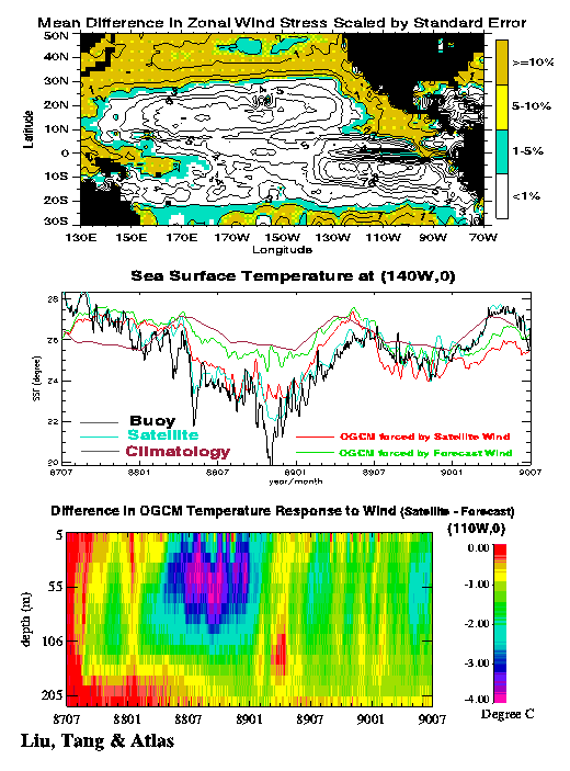
Satellite observations, in situ measurements, and model simulations are combined to assess the oceanic response to surface wind forcing in the equatorial Pacific. The surface wind fields derived from observations by the spaceborne Special Sensor Microwave Imager (SSMI) and from the operational products of the European Centre for Medium Range Weather Forecasts (ECMWF) are compared. The top figure shows significant mean difference between the two wind-stress fields. When SSMI winds are used to force a primitive-equation ocean general circulation model (OGCM), they produce 3C more surface cooling than ECMWF winds for the eastern equatorial Pacific during the cool phase of an El Niño Southern Oscillation (ENSO) event, as shown in the middle figure. The stronger cooling by SSMI winds is in good agreement with measurements at the moored buoys and observations by the Advanced Very High Resolution Radiometer (AVHRR). While the most significant wind differences are found off the equator (centered at 15N and 5S), the largest differences in ocean temperature responses are found on the equator and below the surface (as shown in the bottom figure). The bottom figure, together with the heat budget analysis using OGCM simulated data under different winds, infers that vertical heat advection and uplifting of the thermocline are the dominant factors in the anomalous cooling of the ocean mixed layer. The results of this study indicate that the spacebased winds are superior to winds from weather prediction model in forcing realistic oceanic response, particularly the sea surface anomalies during an ENSO event. The study demonstrates certain maturity and also deficiency in OGCM, and identifies the dominant mechanism for anomalous upper ocean cooling in the 1980s (which may be different from the events in 1990s as discussed by Liu et al., 1996, Eos, 76, 429 and 437). It is an example of combining spacebased ocean observing sensors and OGCM for significant contribution to our understanding of seasonal-to-interannual variability and predictability.
Figure Caption
The top figures shows the distribution of the absolute value of Student's t
which is the mean difference between SSMI and ECMWF zonal wind stresses
divided by the standard error. The areas where the mean difference has
more than 1% probability to come by pure chance from wind stresses of equal
means are colored. The middle figure shows a comparison of first-level
(5-m) temperatures produced by the OGCM, when forced by SSMI and ECMWF
winds, with AVHRR and buoy SST at a location along the equator. The
climatological annual cycle derived from the AVHRR SST is also shown. The
bottom figure shows the time-depth variation of the difference between OGCM
temperature simulations under SSMI and ECMWF winds.